![]()
Introduction to Rydiqule
RydIQule, the Rydberg Interactive Quantum Module, is a python library built to simulate the interaction of Rydberg atoms and light using a semi-classical approach. This notebook will illustrate some of its core functionality, and demonstrate how to use the tool to model simple systems. The intent here is not to demonstrate discoveries in physics, or even simulate useful physics generally. The values provided are deliberately simple integers to make the functions as easy to understand as possible. Thus, the notebook will use cartoonish but nontrivial (from a code perspective) examples to demonstrate how to use the module. Feel free to run the cells of this notebook as-is, but also by all means add and modify cells to get a better feel for how the package works.
This notebook can be downloaded here.
The functionality and principles behind rydiqule are detailed much more thoroughly in the documentation. A few places in the docs are worth pointing out:
API Documentation contains detailed information about how the functions of rydiqule behave from a software perspective.
Physics Documentation contains writeups detailing the physics and math conventions used by rydiqule. There are places where
rydiqulediverges from the conventions of atomic physicists for numerical or code-related reasons, or makes explicit decisions about conventions that are not universal. It is a very helpful reference when something is not working as you expect.There are example notebooks that can be accessed from the docs homepage which contain more realistic use cases for rydiqule.
Design philosophy
Rydiqule was built with a few core principles in mind:
Rydiqule is simple - Setting and solving an atomic system can be done with just a handful of lines of code while behaving in an intuitive way.
Rydiqule is fast - Under the hood, the library makes broad use of fast numpy matrix broadcasting and compiled code in places that would be slowed down by native python. The result is a toolbox that can produce meaningful results in a few minutes or less. This is especially true for steady-state solutions which can be extremely fast, even for large parameter spaces. With version 2.2.0, we introduced a fully compiled time-solver backend that significantly improved time-dependent solve times, bringing them more in line with what is fundamentally achievable.
Rydiqule is flexible - Rydiqule can model a huge variety of semiclassical Rydberg atomic systems with no code modification. For users with more particular modelling needs who wish to extend Rydiqule, the
Sensorclass provides a minimal physical system that can easily be inherited and overloaded for more involved experimental setups (such asCell, which provides an ARC-integrated wrapper toSensorfor calculating Rydberg physics using atomic properties and lab-measured parameters).
Limitations
While we have worked hard to make Rydiqule as good as possible, there are some areas that can cause issues:
Memory -
rydiqule’s speed primarily comes at the cost of increased memory footprint. In order to avoid Python interpreter overhead and fully leverage the speed of Numpy broadcasting and C-level for-looping when solving multiple sets of parameters, we have to pass all equations of motion as a single tensor object to the low-level C functions (such as those backingnumpy.linalg.solveused by the steady-state solver). For systems with many laser parameter values, many levels, doppler averaging in several dimensions, or especially a combination of these, the equations of motion generated by rydiqule are very large, often requiring more memory than is in a typical laptop or simple desktop. For very large systems, the memory footprint may even outpace a powerful workstation. Rydiqule has built-in functionality to handle this, but it is not fully general and it will lead to slower solves.Speed - While huge improvements have been made in the speed of
rydiqulesince its alpha stages, there are certain situations that can still cause slowdowns. For longer time-dependent simulations with large detunings, in particular for the poorly-conditioned equations produced with large doppler width, solving can still be slow. With version 2.2.0, we introduced a fully compiled time-solver backend that greatly improves performance in these situations, but the fundamental time-dependence from large detunings is still present, bounding time-dependent solver performance relative to steady-state solving. Further improvements can be gained from algorithmic developments (such as Floquet techniques), but they typically enforce constraints on the time-dependence that can be modeled.Quantum Back-action - We treat the optical fields as static, and do not include them explicitly in the semi-classical equations of motion. Rydiqule does not account for atom-field back-action effects. This approximation is valid for low optical depth samples, and is known to give valid results for SNR in moderate optical depth samples. However, for quantitative analysis of quantum noise in high optical depth samples, Rydiqule may not be accurate. By extension, rydiqule is also not presently suitable for simulations involving single-photon-level fields.
Device Modelling - Rydiqule is a physics solver, and does not currently have user-friendly support for device-level modelling. Put another way, rydiqule requires a certain level of atomic physics understanding to ensure results are physically meaningful/correct.
Imports
Rydiqule is conventionally imported as rq. In addition, numpy and matplotlib are almost always useful to have in notebooks using rydiqule, so we will import them as well. They are dependencies of rydiqule, so they should already be installed if you installed rydiqule.
import rydiqule as rq
import numpy as np
import matplotlib.pyplot as plt
1. The Sensor object
The Sensor is the core object of rydiqule. It defines an atomic system, and while you can create and solve a Hamiltonian manually, the Sensor takes care of the bookeeping to generate Hamiltonians and solve its associated equations of motion.
Note: Don’t think too hard about why it is called a Sensor, it is a legacy name that does not necessarily capture its entire functionality.
1.1 The quantum state basis of Sensor
The base Sensor class is constructed with a single required argument, which specifies which states are in the basis. Here we create a 3-level system in the manner rydiqule supports: an integer defining the basis size. On its own, a Sensor contains no information about atomic structure; it is an abstraction that allows for a high degree of manual configuration.
basis_size = 3
simple_sensor = rq.Sensor(basis_size)
This is the simplest way to define a Sensor with a particular number of states (3 in this case). In this case, the basis states will simply be labeled [0,1,2], (\(|0\rangle , |1\rangle , |2\rangle\)). However, mutiple other ways exist to label the basis states. Rather than an integer (which will implcitly use python’s range()), we can pass a list of basis state labels directly. These labels can either be strings or tuples. Tuples in particular can be useful for representing quantum numbers, although they can represent anything that you think is useful; they do not invoke any physics in Sensor.
string_sensor = rq.Sensor(['g', 'e1', 'e2'])
tuple_sensor = rq.Sensor([(0,0), (1,-1), (1,0), (1,1)])
Once we have created a Sensor, we can use the Sensor.states attribute to see the states. Note that the ordering of states in a Sensor will always be as they are provided in the constructor.
print(simple_sensor.states)
print(string_sensor.states)
print(tuple_sensor.states)
[0, 1, 2]
['g', 'e1', 'e2']
[(0, 0), (1, -1), (1, 0), (1, 1)]
Specifications of tuples like the one above can become cumbersome, especially to represent large groups of states. For tuples, rydiqule also supports “state specifications”, in which one of the tuple elements is provided as a list. rydiqule will automatically expand such a state into a list as demonstrated below. Note that even when a specification like this is used, it is still necessary to enclose it in list brackets in the constructor. Furthermore, it is often useful to define tuples outside functions, since the number of brackets and parentheses can become cumbersome. This is a safe operation since tuples in python are immutable.
g = (0,0)
e = (1, [-1,0,1])
state_spec_sensor = rq.Sensor([g,e])
print(state_spec_sensor.states)
[(0, 0), (1, -1), (1, 0), (1, 1)]
1.2 Sensor Data structure: The Graph
Before we proceed to useful physics, it is worth a brief sidebar to discuss how the information about levels and couplings is stored in a Sensor. NetworkX is a library for storing and analyzing graphs in python that uses dictionaries to store information about nodes and edges. At the core of a Sensor is a networkx graph. The energy levels in an atomic system are stored as nodes and the couplings between states are stored as edges. Above, when we define a “3-level system”, what rydiqule has created under the hood is a networkx directed graph with 3 nodes and no edges. We can access this graph to view information about it with the Sensor.couplings attribute. Let’s inspect the tuple_sensor we made above and see that the graph nodes are indeed the states we printed above.
print(tuple_sensor.couplings)
print(tuple_sensor.couplings.nodes)
DiGraph with 4 nodes and 0 edges
[(0, 0), (1, -1), (1, 0), (1, 1)]
Indeed the states attribute is just a wrapper for couplings.nodes. Note that this is provided only as an interface to view the graph, and it shoud NOT be modified directly, as doing so may cause rydiqule to either Error or not work as expected.
1.3 Coupling states with simple electromagnetic fields:
While its great to create basis states, there isn’t any physics in an atomic system of completely uncoupled basis states. Fortuntely, it is easy to couple states together in rydiqule to start moddelling interesing physics. States are coupled together using, at minimum, the following:
A 2-element tuple representing the states to be coupled.
The rabi_frequency.
rydiquletreats all frequencies in Mrad/s.The detuning (for couplings to be treated in the rotating frame), or the transition frequency.
Notes on detunings and rotating wave transformation
When we define detunings, the states in a coupling are always defined to go from lower to higher energy. For example, (1,2) means state 2 is higher than 1. Any coupling with a defined detuning will be treated in a rotating frame, with positive detuning always treated as a blue detuning. For now, we will only consider detunings, but later we will discuss transition frequency specification in the cotext of exactly modelling time-dependant effects.
Here we will demonstrate defining a few different systems, showing different equivalent methods for each.
Defining a simple Ladder system
This demonstrates how a minimal ladder system with simple values might be defined in rydiqule. Here we use the standard integer basis and the add_couplings method.
ladder_sensor = rq.Sensor(3)
laser_01 = {"states": (0,1), "detuning": 1, "rabi_frequency": 3}
laser_12 = {"states": (1,2), "detuning": 2, "rabi_frequency": 5}
ladder_sensor.add_couplings(laser_01, laser_12)
To demonstrate what happens under the hood, let us inspect the Sensor.coupling object again, this time looking at the graph edges. We can look at just edges, for an overview of which nodes are coupled, or we can use edges(data=...) for more thorough representations.
print("Edge Keys: ", ladder_sensor.couplings.edges)
print("Edge Data: ", ladder_sensor.couplings.edges(data=True))
print("Edge Rabi: ", ladder_sensor.couplings.edges(data="rabi_frequency"))
Edge Keys:  [(0, 1), (1, 2)]
Edge Data:  [(0, 1, {'rabi_frequency': 3, 'detuning': 1, 'phase': 0, 'kvec': (0, 0, 0), 'coherent_cc': 1.0, 'label': '(0,1)'}), (1, 2, {'rabi_frequency': 5, 'detuning': 2, 'phase': 0, 'kvec': (0, 0, 0), 'coherent_cc': 1.0, 'label': '(1,2)'})]
Edge Rabi:  [(0, 1, 3), (1, 2, 5)]
As we can see, the options described above are just the minimum; there are more keywords we can use to describe a coupling between two states. More complicated uses will be discussed in detail in other places in this notebook, but here is a brief overview of each optimal argument:
phasedescribes the relative phase of a field, and will scale the corresponding off-diagonal terms with an \(e^{i\theta}\) phase offset.kvecis a description of a laser’s k-vector, and is described by (x,y,z) components. This is relevant when we discuss doppler-broadened calculations later. For now, leaving it at the default will ignore doppler effects.coherent_ccis a general abstraction of what is essentially a Clebsch-Gordon coefficient. These will become relevant when we discuss coupling manifolds of states later. The default is 1, and that will effectively ignore the value.labelis a string shorthand that can reference the coupling in some other contexts. Useful labels might include"blue","red","probe","pumping". This label will enforce nothing with regards to physics, but may be helpful. If it is not supplied, it will default to a string cast of the tuple describing the states, as above.
Any of these values can be defined in the coupling in the exact same manner as “detuning” or “rabi_frequency”.
Printing Sensor Data
Since calling that info above is a little bit tedious, rydiqule also supports directly printing a sensor using python’s print() function, which will summarize basic information about a Sensor. We will typically use this method of displaying information about the graph in these notebooks, since it prints in a more readable way.
print(ladder_sensor)
<class 'rydiqule.sensor.Sensor'> object with 3 states and 2 coherent couplings.
States: [0, 1, 2]
Coherent Couplings:
    (0,1): {rabi_frequency: 3, detuning: 1, phase: 0, kvec: (0, 0, 0), coherent_cc: 1.0, label: (0,1)}
    (1,2): {rabi_frequency: 5, detuning: 2, phase: 0, kvec: (0, 0, 0), coherent_cc: 1.0, label: (1,2)}
Decoherent Couplings:
    None
Energy Shifts:
    None
We will discuss Decoherent Couplings and Energy shifts, later, but for now we can see this is a substantially easier way to view information about the Sensor
Automatic Hamiltonian generation
Once the system is defined, we can see the Hamiltonian matrix. In many ways, this is the core piece of rydiqule that makes it useful. You usually will not need to call this explicitly (it will be called internally by a solver, more on that later), but it can be useful to make sure the system is defined as expected.
print(ladder_sensor.get_hamiltonian())
[[ 0. +0.j  1.5+0.j  0. +0.j]
 [ 1.5-0.j -1. +0.j  2.5+0.j]
 [ 0. +0.j  2.5-0.j -3. +0.j]]
Note the detuning sign convention. We have added a positive detuning value to the system. rydiqule chooses a rotating frame automatically, and there is no user-configurable option to change it. The roating frame chosen is one in which a detuning of 1 corresponds to an term of -1 on the Hamiltonian diagonal.
Defining a simple Vee scheme
We can do something similar, but with a different arrangement of couplings, and using explicit strings to define the basis. We can also pass fields in the constructor if we like.
basis = ["g", "e1", "e2"]
laser_01 = {"states": ("g","e1"), "detuning": 1, "rabi_frequency": 3, "label":"red"}
laser_02 = {"states": ("g","e2"), "detuning": 2, "rabi_frequency": 5, "label":"blue"}
sensor_v = rq.Sensor(basis, laser_01, laser_02)
print(sensor_v.couplings.edges(data="label"))
print(sensor_v.get_hamiltonian())
[('g', 'e1', 'red'), ('g', 'e2', 'blue')]
[[ 0. +0.j  1.5+0.j  2.5+0.j]
 [ 1.5-0.j -1. +0.j  0. +0.j]
 [ 2.5-0.j  0. +0.j -2. +0.j]]
Defining a simple Lambda scheme
Here is another system, this time a lambda scheme. Here we demonstrate another way to add couplings using the add_coupling function. This function behaves equivalently to add_couplings, and which you choose is up to preference.
As one final way of defing our basis, let’s use tuples here. This can be a little more involved, but occasionally useful in large sytems. As discussed above, we will alias the states so couplings don’t start getting clunky to define. We also show the expand_statespec function to turn the e variable into a list of all possible values.
g = (0,0)
e = (1, [-1,0,1])
print("e states: ", rq.expand_statespec(e)) #just creates a list, no physics is done here
[e1, e2, e3] = rq.expand_statespec(e) #unpack the list for easy use later.

sensor_lambda = rq.Sensor([g, e]) #note that ryqiqule will automatically unpack e into a list

sensor_lambda.add_coupling((g, e1), rabi_frequency=1, detuning=1)
sensor_lambda.add_coupling((e1,e2), rabi_frequency=2, detuning=2)
sensor_lambda.add_coupling((e3,e2), rabi_frequency=3, detuning=3) #tuples always go from low to high energy by convention

print(sensor_lambda)
print(sensor_lambda.get_hamiltonian())
e states:  [(1, -1), (1, 0), (1, 1)]
<class 'rydiqule.sensor.Sensor'> object with 4 states and 3 coherent couplings.
States: [(0, 0), (1, -1), (1, 0), (1, 1)]
Coherent Couplings:
    ((0, 0),(1, -1)): {rabi_frequency: 1, detuning: 1, phase: 0, kvec: (0, 0, 0), coherent_cc: 1.0, label: ((0, 0),(1, -1))}
    ((1, -1),(1, 0)): {rabi_frequency: 2, detuning: 2, phase: 0, kvec: (0, 0, 0), coherent_cc: 1.0, label: ((1, -1),(1, 0))}
    ((1, 1),(1, 0)): {rabi_frequency: 3, detuning: 3, phase: 0, kvec: (0, 0, 0), coherent_cc: 1.0, label: ((1, 1),(1, 0))}
Decoherent Couplings:
    None
Energy Shifts:
    None
[[ 0. +0.j  0.5+0.j  0. +0.j  0. +0.j]
 [ 0.5-0.j -1. +0.j  1. +0.j  0. +0.j]
 [ 0. +0.j  1. -0.j -3. +0.j  1.5-0.j]
 [ 0. +0.j  0. +0.j  1.5+0.j  0. +0.j]]
Systems that are not fully coupled
We can also define a system in which not all states are connected explicitly by couplings. This allows us to solve systems which, for example, have states coupled only by decoherence. This exact use case will be demonstrated later, but we can set up the system and show the hamiltonian here.
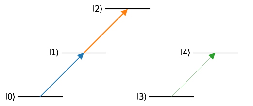
The hamiltonaian works by treating an uncoupled states as a “second ground state”, and calculates digonal hamiltonian elements from there. We show a 4-level system in which state 4 is coupled to state 5 via a steady state rf transition, but to no other states. It should be noted that calling an rf transition does not change the way the system is solved here.
Looking at the hamiltonian, we can see that the 4th term along the diagonal is 0, and the 5th term counts from there.
sensor_uncoupled = rq.Sensor(5)
laser_01 = {"states": (0,1), "detuning": 1, "rabi_frequency": 3}
laser_12 = {"states": (1,2), "detuning": 2, "rabi_frequency": 5}
rf = {"states": (3,4), "detuning": 8, "rabi_frequency": 1}
sensor_uncoupled.add_couplings(laser_01, laser_12, rf)

print(sensor_uncoupled.get_hamiltonian())
[[ 0. +0.j  1.5+0.j  0. +0.j  0. +0.j  0. +0.j]
 [ 1.5-0.j -1. +0.j  2.5+0.j  0. +0.j  0. +0.j]
 [ 0. +0.j  2.5-0.j -3. +0.j  0. +0.j  0. +0.j]
 [ 0. +0.j  0. +0.j  0. +0.j  0. +0.j  0.5+0.j]
 [ 0. +0.j  0. +0.j  0. +0.j  0.5-0.j -8. +0.j]]
In some more complicated cases, we may want a more concrete visual reassurance that everything is defined correctly. rydiqule makes use of the leveldiagram library (which uses matplotlib as a backend) to help draw visual representations of a Sensor. In the drawing below, we can see that the diagram indeed shows that states 2 and 3 are not coupled. Keep in mind that these drawings have limitations. Especially in very large, highly-coupled systems, the output can get quite cramped, although it is still a helpful sanity check.
rq.draw_diagram(sensor_uncoupled)
<leveldiagram.ld.LD at 0x2333b297dd0>
1.5 Coupling state manifolds
So far we have shown the basics of adding couplings. There is one final important detail regard coherent couplings, and that is the use of add_coupling to couple entire groups of states with a single call. To do so, we define a statespec as in the Lambda example above. Let’s construct a similar Sensor.
g = (0,0)
e = (1, [-1,0,1])
[e1, e2, e3] = rq.expand_statespec(e)

sensor_man = rq.Sensor([g, e])
print(sensor_man.couplings.nodes)
[(0, 0), (1, -1), (1, 0), (1, 1)]
Once we have the Sensor defined, we can actually couple the ground state to every excited state with a single call by simply treating e as one state. Note that in this case, "label" becomes a required argument. Defining in this way will automagically loop over every state in the e “manifold” and add a coupling between g and each one. Let’s add the coupling and see what edges get added.
sensor_man.add_coupling((g,e), rabi_frequency=2, detuning=1, label="probe")
print(sensor_man)
<class 'rydiqule.sensor.Sensor'> object with 4 states and 3 coherent couplings.
States: [(0, 0), (1, -1), (1, 0), (1, 1)]
Coherent Couplings:
    ((0, 0),(1, -1)): {rabi_frequency: 2, detuning: 1, phase: 0, kvec: (0, 0, 0), label: probe_0, coherent_cc: 1.0}
    ((0, 0),(1, 0)): {rabi_frequency: 2, detuning: 1, phase: 0, kvec: (0, 0, 0), label: probe_1, coherent_cc: 1.0}
    ((0, 0),(1, 1)): {rabi_frequency: 2, detuning: 1, phase: 0, kvec: (0, 0, 0), label: probe_2, coherent_cc: 1.0}
Decoherent Couplings:
    None
Energy Shifts:
    None
Note that as-is, these 3 states are degenerate. There are a few modifications we can make.
We can use the
add_energy_shiftsfunction to break the degeneracy. This will have the effect of adding diagonal terms to the hamiltonian.Now the
coherent_ccwe saw above becomes relevant. We can add a dictionary that represents a “weighting” to each individual coupling in the group, and pass it under the “coupling_coefficients” keyword. This will not change the rabi_frequency directly, but it will apply a prefactor to the rabi_frequency when generating the hamiltonian.
We will re-make the sensor, and make some sensible choices to demonstate energy_shifts and coupling_coefficients, in this case using dictionaries. Take a moment to understand this part: it is crucial to understand how to do more advanced calculations. Here we also see where the Energy Shifts section of the printout comes in.
g = (0,0)
e = (1, [-1,0,1])
[e1, e2, e3] = rq.expand_statespec(e)

#defing coupling coefficients and energy shifts
cc = {
    (g,e1): 0.25,
    (g,e2): 0.5,
    (g,e3): 0.25
}
e_shifts = {e1:-0.1, e3: 0.1}
sensor_man = rq.Sensor([g, e])
sensor_man.add_energy_shifts(e_shifts)
sensor_man.add_coupling((g,e), detuning=1, rabi_frequency=2, coupling_coefficients=cc, label="foo")

print(sensor_man)
<class 'rydiqule.sensor.Sensor'> object with 4 states and 3 coherent couplings.
States: [(0, 0), (1, -1), (1, 0), (1, 1)]
Coherent Couplings:
    ((0, 0),(1, -1)): {rabi_frequency: 2, detuning: 1, phase: 0, kvec: (0, 0, 0), label: foo_0, coherent_cc: 0.25}
    ((0, 0),(1, 0)): {rabi_frequency: 2, detuning: 1, phase: 0, kvec: (0, 0, 0), label: foo_1, coherent_cc: 0.5}
    ((0, 0),(1, 1)): {rabi_frequency: 2, detuning: 1, phase: 0, kvec: (0, 0, 0), label: foo_2, coherent_cc: 0.25}
Decoherent Couplings:
    None
Energy Shifts:
    (1, -1): -0.1
    (1, 1): 0.1
One thing to note here is that e_shift actually adds an edge from a node to itself. This isn’t a crucial detail, but can be helpful to know if you need to debug a complicated system. Now that everything on the graph makes sense, lets see what the Hamiltonian does:
print(sensor_man.get_hamiltonian())
[[ 0.  +0.j  0.25+0.j  0.5 +0.j  0.25+0.j]
 [ 0.25-0.j -1.1 +0.j  0.  +0.j  0.  +0.j]
 [ 0.5 -0.j  0.  +0.j -1.  +0.j  0.  +0.j]
 [ 0.25-0.j  0.  +0.j  0.  +0.j -0.9 +0.j]]
We have broken the energy level degeneracy with some terms added along the diagonal, and given a stronger coupling to the (1,0) state.
1.6 Decoherent transitions
There is one more important aspect of defining the Sensor graph that we have not discussed (which we can actually see as absent in theSensor printout), and that is decoherent couplings. Decays of this sort are added with the add_decoherence function, which works very similarly to the add_coupling function. State manifolds and coupling coefficients work in an identical manner. Here we can copy the Sensor we used above, and add a decoherence in coupling the excited manifold to the ground state. The only minor difference is that decoherences do not use keyword arguments, but added with a single required argument defining the decay rate, again in Mrad/sec.
g = (0,0)
e = (1, [-1,0,1])
[e1, e2, e3] = rq.expand_statespec(e)

#defing coupling coefficients and energy shifts
cc = {
    (g,e1): 0.25,
    (g,e2): 0.5,
    (g,e3): 0.25
}
e_shifts = {e1:-0.1, e3: 0.1}

sensor_man = rq.Sensor([g, e])
sensor_man.add_energy_shifts(e_shifts)
sensor_man.add_coupling((g,e), detuning=1, rabi_frequency=2, coupling_coefficients=cc, label="foo")
sensor_man.add_decoherence((e,g), 0.1, label="bar")
print(sensor_man.get_hamiltonian())
[[ 0.  +0.j  0.25+0.j  0.5 +0.j  0.25+0.j]
 [ 0.25-0.j -1.1 +0.j  0.  +0.j  0.  +0.j]
 [ 0.5 -0.j  0.  +0.j -1.  +0.j  0.  +0.j]
 [ 0.25-0.j  0.  +0.j  0.  +0.j -0.9 +0.j]]
Obviously, the hamiltonian will be the same, but we can inspect what got added to the graph again using Sensor.couplings.edges. We will then get the decoherence matrix with decoherence_matrix, similarly to get_hamiltonian(). We will discuss how the decoherence matrix is used in more detail below when we discuss solving.
print("Graph Edges: ")
print(sensor_man.couplings.edges(data=True))
print("Decoherence matrix: ")
print(sensor_man.decoherence_matrix())
Graph Edges:
[((0, 0), (1, -1), {'rabi_frequency': 2, 'detuning': 1, 'phase': 0, 'kvec': (0, 0, 0), 'label': 'foo_0', 'coherent_cc': 0.25}), ((0, 0), (1, 0), {'rabi_frequency': 2, 'detuning': 1, 'phase': 0, 'kvec': (0, 0, 0), 'label': 'foo_1', 'coherent_cc': 0.5}), ((0, 0), (1, 1), {'rabi_frequency': 2, 'detuning': 1, 'phase': 0, 'kvec': (0, 0, 0), 'label': 'foo_2', 'coherent_cc': 0.25}), ((1, -1), (1, -1), {'e_shift': -0.1, 'label': '(1, -1)'}), ((1, -1), (0, 0), {'gamma_bar': 0.1, 'label': '((1, -1),(0, 0))'}), ((1, 0), (0, 0), {'gamma_bar': 0.1, 'label': '((1, 0),(0, 0))'}), ((1, 1), (1, 1), {'e_shift': 0.1, 'label': '(1, 1)'}), ((1, 1), (0, 0), {'gamma_bar': 0.1, 'label': '((1, 1),(0, 0))'})]
Decoherence matrix:
[[0.  0.  0.  0. ]
 [0.1 0.  0.  0. ]
 [0.1 0.  0.  0. ]
 [0.1 0.  0.  0. ]]
The edges are getting quite busy, but we will spot "gamma_bar" attributes on the expected graph edges. This is the convention used by rydiqule: when add_decoherence or a related function is called, and label is provided, the associated key on the graph will be "gamma_" + label. If no label is provided, simply "gamma" will be used for the key. When decoherence_matrix is called, every attribute on each edge that starts with "gamma" will be added together and placed on the appropriate term of a decoherence matrix.
There are a few more functions to be aware of when it comes to definining decoherence rates:
add_transit_broadeningwill add a decoherence from each state to the ground state (by default) or to a particular set of ground states. This function is designed to account for atoms which move out of a laser and are replaced by atoms in their ground state(s). Fractional transit broadenings are specified with therepopkeyword arg.add_self_broadeningwill add a decoherence from a state to itself to account for a atoms losing coherence; remaining in the same state.set_gamma_matrixtakes a square numpy array as an argument, then applies an appropriate"gamma"value to each graph edge.
We have printed attributes directly from the graph for the purposes of demonstrating what is happening under the hood. Unless you need to inspect attributes of the graph directly, a simple print statement will give us a more readable output.
print(sensor_man)
<class 'rydiqule.sensor.Sensor'> object with 4 states and 3 coherent couplings.
States: [(0, 0), (1, -1), (1, 0), (1, 1)]
Coherent Couplings:
    ((0, 0),(1, -1)): {rabi_frequency: 2, detuning: 1, phase: 0, kvec: (0, 0, 0), label: foo_0, coherent_cc: 0.25}
    ((0, 0),(1, 0)): {rabi_frequency: 2, detuning: 1, phase: 0, kvec: (0, 0, 0), label: foo_1, coherent_cc: 0.5}
    ((0, 0),(1, 1)): {rabi_frequency: 2, detuning: 1, phase: 0, kvec: (0, 0, 0), label: foo_2, coherent_cc: 0.25}
Decoherent Couplings:
    ((1, -1),(0, 0)): {gamma_bar: 0.1}
    ((1, 0),(0, 0)): {gamma_bar: 0.1}
    ((1, 1),(0, 0)): {gamma_bar: 0.1}
Energy Shifts:
    (1, -1): -0.1
    (1, 1): 0.1
2. Solving a Sensor in the steady-state case
So far we have just created sensor objects and shown their corresponding Hamiltonians. The most important functionality of rydiqule, however, is solving their associated equations of motion automatically. Here we will demonstrate some of the ways to solve a simple system using rydiqule.
2.1 What is rydiqule actually solving?
In the section title, we simply refer to “solving a sensor”. When we discuss solving a system, what we mean is that we are solving the Lindblad Master Equation associated with the system described by our Sensor:
where \(\mathcal{L}\) is the Lindblad operator that accounts for non-unitary dephasing effects.
When rydiqule solves in the steady state, what is ultimately produced is the steady-state solution of that differential equation. rydiqule is capable of inferring the relevant matrix quantities from the graph defined by a Sensor, as we have seen above.
2.2 Basic Solving in the steady state
If all we need is steady state behavior of a particular system, it is straightforward and quick in rydiqule. By wrapping a simple matrix differential equation solver, rydiqule can quickly get the steady state frequencies of each element of the density matrix \(\rho\) of the system. We start by re-defining the same ladder system we had at the beginning of the notebook.
basis_size = 3
sensor_demo = rq.Sensor(basis_size)

laser_01 = {"states": (0,1), "detuning": 1, "rabi_frequency": 3}
laser_12 = {"states": (1,2), "detuning": 2, "rabi_frequency": 5}
sensor_demo.add_couplings(laser_01, laser_12)

gamma = np.zeros((basis_size, basis_size))
gamma[1:,0] = 0.1
print(gamma)
sensor_demo.set_gamma_matrix(gamma)
[[0.  0.  0. ]
 [0.1 0.  0. ]
 [0.1 0.  0. ]]
Now, instead of showing the Hamiltonian, we can just call the rydiqule.solve_steady_state() function on sensor and get the result.
solution_demo = rq.solve_steady_state(sensor_demo)
print(solution_demo)
<rydiqule.sensor_solution.Solution object at 0x000002333B42EE40>
2.3 The Solution object
As you can see, the solution itself is not an array, but an object containing some extra information. When rydiqule solves a system, it saves the solution, but also many other things relevant to the solve (including the graph itself), so that relevant quantities about the original Sensor and solve can be computed and reproduced. Since the above output is a bit cluttered, let’s contain outselves to just the important quanties for now. First, couplings is just a copy of the Sensor.couplings graph discussed above for the Sensor on which solve_steady_state was called. Next, rho is the density matrix solution of the system, but there is a catch.
print(f"Couplings: {solution_demo.couplings}")
print(f"rho: {solution_demo.rho}")
print(len(solution_demo.rho))
Couplings: DiGraph with 3 nodes and 4 edges
rho: [-0.09225689 -0.1820376   0.01617957  0.27218216  0.21003648  0.00831697
  0.0042641   0.21320497]
8
Adjustments to the equations
So why does the solution have 8 elements? Why is it real? Why is it 1-dimensional? After all, it represents a density matrix, which should have \(n^2\) complex-valued elements (\(3^2=9\) in this case), ideally arranged in square.
For numerical stability, rydiqule removes the ground state population equations, so the \(\rho_{00}\) term is omitted from the solution (typically \(\rho_{00} >> \rho_{ij}\) for \(ij \neq 00\), which is the source of the numerical problems). If needed, it can be inferred as \(\rho_{00} = 1 - \sum_{i=1}^{n} \rho_{ii}\). Furthermore, rydiqule transforms the basis so that all values are real. Rather than an \(n\times n\) Hermitian matrix, rydiqule parameterizes the density matrix \(\rho\) as \(n\times n\) real values before removing the ground state, for a total of \(n^2-1\) values. For more details, refer to the documentation. We really do wish these modifications were not necessary, but keeping the ground state population and complex density matrix elememts resulted in unphysical soulutions during development.
So how do we know (ideally quickly) which element of the solution corresponds to which density matrix element? The Solution contains an attribute called dm_basis which does exactly this, containing a list of strings showing the info we want. Since the density matrix is hermitian and trace 1, this array does indeed contain all of the information of the density matrix. Note that dm_basis does not include \(\rho_{00}\) since the ground state is removed by the solver.
We choose to keep this basis in rydiqule since it is more transparent to what rydiqule does under the hood, and is used in further calculations.
print(solution_demo.dm_basis)
['10_real' '20_real' '10_imag' '11_real' '21_real' '20_imag' '21_imag'
 '22_real']
If we quickly want a particular full complex density matrix element, the rho_ij function does precisely that:
print(f"rho_10 = {solution_demo.rho_ij(1,0)}")
rho_10 = (-0.09225688789212251+0.016179570807727885j)
There are a few other functions to be aware of in a Solution object. Some commonly-computed quantities that might be derived from a density matrix solution. Before we discuss them, it is worth a brief aside on the Solution.probe_tuple quantity. It is a quantity that is derived from the Sensor that is the transition over which, by default, observable calculations will be made. So in the absence of any other information, when observable values are computed, they are computed for the density matrix elements that are defined by the probe_tuple. The probe_tuple is set by the first coupling that is added with the add_coupling function in Sensor (equivalently, the first dictionary passed to add_couplings). While this quantity can be set manually, it is usually better practice to define whatever the probing transition (usually the laser you will be measuring) first, and not change probe_tuple manually when it can be avoided. To demonstrate this, we can see what probe_tuple is in both the Sensor and Solution.
print(sensor_demo.probe_tuple)
print(solution_demo.probe_tuple)
(0, 1)
(0, 1)
As expected, this is the the first coupling added to the system. Below is a (very) brief example to show the probe_tuple being added.
sensor_probe = rq.Sensor(3)
print(sensor_probe.probe_tuple)
sensor_probe.add_coupling((0,2), rabi_frequency=1, detuning=0)
print(sensor_probe.probe_tuple)
sensor_probe.add_coupling((1,2), rabi_frequency=1, detuning=0)
print(sensor_probe.probe_tuple)
None
(0, 2)
(0, 2)
With the probe_tuple cleared up, we can explore a few of the other functions in a Solution.
get_observable(A)is a function which, given an observable matrix \(A\), uses the density matrix definition of the expectation value of \(A\), \(\langle A\rangle = tr(\rho A)\).coupling_coefficent_matrix(<coupling>)returns a matrix of all coupling coefficients on a particular transition defined by coupling. We discussed the coupling cofficients above in the context of relative coupling strength. In this way they can be thought of as a unitless analogue of the dipole moment.Given these two quantities, you may be developing an idea that it my be useful to pass the output of
coupling_coefficient_matrixtoget_observableand use that to compute susceptibility. It’s such a good idea,rydiqulewent ahead and implemented that function inSolution.get_susceptibility(). The value will be computed from a handful of quantities built in toSolution, and more details about its calculation can be found in the docs. Note that this calculation will require setting thekappaandprobe_freqattributes in aSensorbefore it is solved (or, technically, in the solution itself but this is not the recommended use). Again, see the docs for further details. Note that this function will implicitly only get the observable over theprobe_tupletransition.
We will demonstrate getting the susceptibility with get_susceptibility() below, although keep in mind these are very cartoonish and unphysical values
sensor_demo.set_experiment_values(kappa=1, probe_freq=1000)
solution_demo = rq.solve_steady_state(sensor_demo)
print(solution_demo.get_susceptibility())
(-0.03687722558481313+0.006467351069111717j)
2.4 Stacking: Solving for multiple values of a parameter
Getting a single result is nice, but really just a single data point. One of the simplest types of experiments you might want to simulate is to scan, for example, over a range of detuning values and see the behavior of the system at each value. One of rydiqule’s greatest strength is its handling of simulations like this. Suppose we wanted to sweep our probe laser detuning between -10 MHz and 10 MHz. Without rydiqule we might write an explicit loop over a set of values, modifying and solving the system at each iteration, and storing the results in a new list. In python especially, this sort of approach has a high computational overhead.
With rydiqule, we can set up the system similarly to above, this time as a 4-level system. However, this time, instead of using a single float value for a coupling parameter, we will define the \(0\leftrightarrow 1\) coupling detunuing value as a 1-dimensional numpy array constructed with the linspace function. after this, rydiqule will handle the rest.
basis_size = 4
sensor_sweep = rq.Sensor(basis_size)

detunings = 2*np.pi*np.linspace(-10,10,201) #201 values between -10 and 10 MHz
probe = {"states":(0,1), "detuning": detunings, "rabi_frequency": 3}
coupling = {"states":(1,2), "detuning": 0, "rabi_frequency": 5}
rf = {"states":(2,3), "detuning": 0, "rabi_frequency":7}

sensor_sweep.add_couplings(probe, coupling, rf)

sensor_sweep.add_decoherence((1,0), 0.1)
sensor_sweep.add_decoherence((2,1), 0.1)
sensor_sweep.add_decoherence((3,0), 0.1)
Before we continue further, let us examine the printout of the Sensor, and the shape of the hamiltonian produced by get_hamiltonian:
print(sensor_sweep)
print(sensor_sweep.get_hamiltonian().shape)
<class 'rydiqule.sensor.Sensor'> object with 4 states and 3 coherent couplings.
States: [0, 1, 2, 3]
Coherent Couplings:
    (0,1): {rabi_frequency: 3, detuning: <parameter with 201 values>, phase: 0, kvec: (0, 0, 0), coherent_cc: 1.0, label: (0,1)}
    (1,2): {rabi_frequency: 5, detuning: 0, phase: 0, kvec: (0, 0, 0), coherent_cc: 1.0, label: (1,2)}
    (2,3): {rabi_frequency: 7, detuning: 0, phase: 0, kvec: (0, 0, 0), coherent_cc: 1.0, label: (2,3)}
Decoherent Couplings:
    (1,0): {gamma: 0.1}
    (2,1): {gamma: 0.1}
    (3,0): {gamma: 0.1}
Energy Shifts:
    None
(201, 4, 4)
Here we see the familiar \(4\times 4\) hamiltonian, but with an additional dimension of size 201, exaclty the size of our detuning array. What rydiqule has done behind the scenes is generate a \(4\times 4\) Hamiltonian matrix for every detuning value in the array and place them all into a single np.ndarray, enabling the use of fast broadcasted numpy functions. rydiqule calls this “stacking”, and it is the key behind rydiqule’s impressive python performace for complicated experiments. Most (although not all) parameters of a Sensor can be scanned in this way. The complete list of scannable parameters is:
detuningrabi_frequencyphasee_shiftAll decoherences
An important note about rydiqule’s internal functions is that they are completely agnostic to what each axis of a stack represents, when run through the internal functions, all it needs to know is that something is a stack of hamiltonians. Equations, or density matrices, and the fuctions that use them are performed identically. This will be an important detail in later sections.
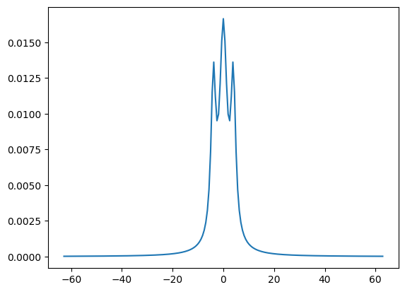
From here, we solve exactly as before. Rydiqule will automagically solve the system for every detuning value (very quickly). We also show the utility function get_rho_ij() which extracts \(\rho_{ij}\) from the density matrix \(\rho\) of any solution (regardless of how many dimensions it is). We use it to get \(\rho_{01}\).
solution = rq.solve_steady_state(sensor_sweep)
print(f"Solution shape: {solution.rho.shape}")
absorption = solution.coupling_coefficient_observable().imag
print(f"Absorption_shape: {absorption.shape}")
Solution shape: (201, 15)
Absorption_shape: (201,)
We can see that there is a 15-element solution for each one of the detuning values. After we get the absorption using get_rho_ij(), we can see that we are left with a single array with 201 elements, corresponding to to the absorption at each value of detuning. Still, that was pretty fast for solving 200 equations. The function doesn’t do anything special, it just is a quick way to get common info you might want out of a solution. We can now do a quick-and-dirty plot to see what it looks like:
plt.plot(detunings, absorption)
plt.show()
2.5 Solving for multiple values of multiple parameters
If you like the simplicity of scanning an single laser detuning in rydiqule, you will be even more excited to learn that rydiqule can handle scans over multple different parameters simulataneously. We will set up the sensor as before, with a couple of changes. We will now also scan the dephasing rate and show how the absorption changes.
basis_size = 4
sensor_sweep_2 = rq.Sensor(basis_size)

detunings = 2*np.pi*np.linspace(-10, 10, 201) #201 values between -10 and 10 MHz
probe = {"states":(0,1), "detuning": detunings, "rabi_frequency": 3, "label":"probe"}
coupling = {"states":(1,2), "detuning": 0, "rabi_frequency": 5, "label": "coupling"}
rf = {"states":(2,3), "detuning": 0, "rabi_frequency":7, "label": "rf"}

sensor_sweep_2.add_couplings(probe, coupling, rf)

gamma10 = np.linspace(0.1, 1.0, 10)
sensor_sweep_2.add_decoherence((1,0), gamma10)
sensor_sweep_2.add_decoherence((2,1), 0.1)
sensor_sweep_2.add_decoherence((3,0), 0.1)

print(sensor_sweep_2)
<class 'rydiqule.sensor.Sensor'> object with 4 states and 3 coherent couplings.
States: [0, 1, 2, 3]
Coherent Couplings:
    (0,1): {rabi_frequency: 3, detuning: <parameter with 201 values>, phase: 0, kvec: (0, 0, 0), label: probe, coherent_cc: 1.0}
    (1,2): {rabi_frequency: 5, detuning: 0, phase: 0, kvec: (0, 0, 0), label: coupling, coherent_cc: 1.0}
    (2,3): {rabi_frequency: 7, detuning: 0, phase: 0, kvec: (0, 0, 0), label: rf, coherent_cc: 1.0}
Decoherent Couplings:
    (1,0): {gamma: <parameter with 10 values>}
    (2,1): {gamma: 0.1}
    (3,0): {gamma: 0.1}
Energy Shifts:
    None
Once again, no extra steps are required, just call solve_steady_state() as normal, and look at the shape of the solution and the absorption and rydiqule will quickly find the solution for every combination of those 2 parameters.
solution_2 = rq.solve_steady_state(sensor_sweep_2)
print(f"Solution shape: {solution_2.rho.shape}")
absorption_2 = solution_2.coupling_coefficient_observable().imag
print(f"Absorption_shape: {absorption_2.shape}")
Solution shape: (201, 10, 15)
Absorption_shape: (201, 10)
How do we know which axis corresponds to the probe detuning and which is the coupling detuning? It is obvious in this case since they are different lengths, but this will not always be the case (for example in cases where two lasers are scanned over the same number of values). Sensor and Solution both have attributes called axis_labels which do just that, and this is where labeling our couplings comes in handy (It is a method of Sensorand an attribute of Solution for reasons that are not important here). Note that if couplings are not labeled, the axes will default to being labeled by the states they couple. For example ["(0,1)_detuning", (1,2)_detuning"], in this case, the output of axis_labels is what we would expect based on the solution shape we printed above. Notice that since the detuning scanned was on the laser we labelled "probe", that label is reflected on the axis.
In the case of a Solution, the axis of the density matrix is included, but this is not the case in Sensor, since there is no associated density matrix until it is solved.
print(sensor_sweep_2.axis_labels())
print(solution_2.axis_labels)
['probe_detuning', '(1,0)_gamma']
['probe_detuning', '(1,0)_gamma', 'density_matrix']
So the first axis corresponds to the probe laser detuning, and the second axis corresponds to \(\Gamma_{1,0}\). Now calling a function like np.argmin() or np.argmax() could quickly be used to optimize some value over a large parameter space. rydiqule lets us add as many parameters as you like as a list, detunings, rabi frequencies, or dephasings. It’s handy, but beware that the memory footprint can quickly balloon out of control when generating equations of motion if you get too ambitious, increasing by a factor of \(n\) when you add an axis with \(n\) elements, especially given that many values used in internal calculations are 128-bit complex arrays.
Currently, rydiqule has internal functions to spot this before it happens and break it into more manageable chunks if it can, but it is certainly possible to make a system which even it cannot handle. If the solution does not fit in memory, no amount of splitting up the equations will allow the system to be solved, and you should reconsider the size of your parameter space. Even in the above example, rydiqule is solving \(201\times 10 \geq 2,000\) equations simultaneously (which is still pretty good). In cases where the parameter space would become intractably large, it is generally good practice to optimise over specific subsets of parameters at a time, or use a coarser mesh to identify a smaller region of interest.
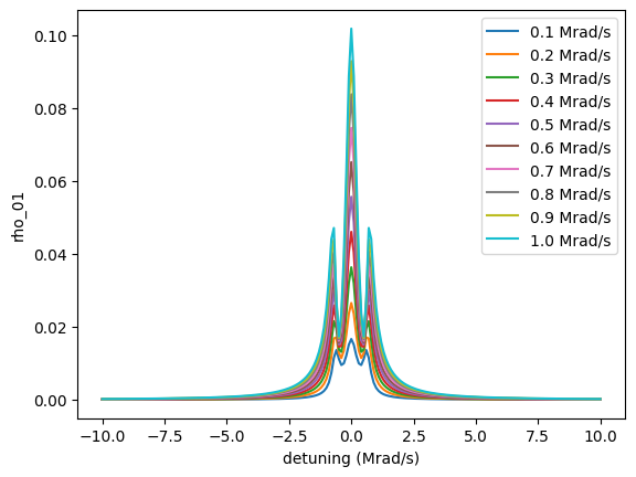
We can plot these probe sweeps at the same time fairly simply.
fig, ax = plt.subplots(1)

for i in range(absorption_2.shape[1]):
    ax.plot(detunings/2/np.pi, absorption_2[:,i], label=f'{gamma10[i]:.1f} Mrad/s')

ax.set_xlabel("detuning (Mrad/s)")
ax.set_ylabel("rho_01")

ax.legend();
fig
2.6 Parameter zipping
It is not uncommon in atomic physics experiments for 2 different atomic transitions (even just among sublevels) to originate from the same laser. In this case, it is often desirable to run simulations where a value of a parameter in one transition (say the laser power/rabi frequency) maps 1-to-1 to a value in a different transition. At the very least, ensuring that these values are always run together will reduce the number of calculations that need to be done substantially by elimnating unphysical simulations.
Zipping Basics
To handle this case, Sensor has a function called zip_parameters. We call it a zip because it can be thought about in the same way that python’s native zip() works for iterators. A zip is defined with a dictionary keyed with coupling labels (including the automatically-generated ones like "(1,2)"). zip_parameters takes this dictionary as an argument, then places all those values on the same axis in the hamiltonian and equation stack. We demonstrate it below:
sensor_zip = rq.Sensor(3)
det = np.linspace(-5,5,101)
f1 = {"states": (0,1), "rabi_frequency": 1, "detuning": det, "label":"laser"}
f2 = {"states": (1,2), "rabi_frequency": 1, "detuning": 2*det}
sensor_zip.add_couplings(f1, f2)
print(f"shape before zip: {sensor_zip.get_hamiltonian().shape}")
sensor_zip.zip_parameters({"laser":"detuning", "(1,2)":"detuning"}, zip_label="foo")
print(f"shape after zip: {sensor_zip.get_hamiltonian().shape}")
shape before zip: (101, 101, 3, 3)
shape after zip: (101, 3, 3)
We labelled the zip as "foo", and this is what will be shown on the output of "axis_labels". Had we not provided a label, the one created would be all the couplings joined with underscores. This can be cumbersome-looking, so it generally good practice to label your zips, although not strictly mandatory.
sensor_zip.add_transit_broadening(0.1)
sol = rq.solve_steady_state(sensor_zip)
print(sol.axis_labels)
['foo', 'density_matrix']
Now all the parameters we zipped should line up on their shared axis. As an example, if we inspect Hamiltonian 0, it should correspond to a detuning of -5 (the first detuning value) on the first coupling and -10 (the first detuning value) on the second:
print(sensor_zip.get_hamiltonian()[0])
[[ 0. +0.j  0.5+0.j  0. +0.j]
 [ 0.5-0.j  5. +0.j  0.5+0.j]
 [ 0. +0.j  0.5-0.j 15. +0.j]]
It is worth noting that zip_parameters does not change anything on the graph itsself, it just adds the labels to a list which is an internal attribute. The actual zipping is done at hamiltonian/decoherence matrix generation time.
Automatic Zipping
When couplings are defined between manifolds of states as shown above (thus producing more than 1 graph edge) any array-like parameters will be zipped automatically. So no additional steps need to be taken, and the shape of the Hamiltonian will be correct. Here, we see that all the detunings are included as arrays on separate edges, but they share an axis on the hamiltonian automatically.
g = (0,0)
e = (1, [-1,0,1])
[e1, e2, e3] = rq.expand_statespec(e)

#defing coupling coefficients and energy shifts
cc = {
    (g,e1): 0.25,
    (g,e2): 0.5,
    (g,e3): 0.25
}
e_shifts = {e1:-0.1, e3: 0.1}

det = np.linspace(-1,1,11) #short array for readable printout

sensor_man_zip = rq.Sensor([g,e])
sensor_man_zip.add_energy_shifts(e_shifts)
sensor_man_zip.add_coupling((g,e), rabi_frequency=2, detuning=det, coupling_coefficients=cc, label="laser")

print(sensor_man_zip)

print(f"Hamiltonian Shape :{sensor_man_zip.get_hamiltonian().shape}")
print(sensor_man_zip.axis_labels())
<class 'rydiqule.sensor.Sensor'> object with 4 states and 3 coherent couplings.
States: [(0, 0), (1, -1), (1, 0), (1, 1)]
Coherent Couplings:
    ((0, 0),(1, -1)): {rabi_frequency: 2, detuning: <parameter with 11 values>, phase: 0, kvec: (0, 0, 0), label: laser_0, coherent_cc: 0.25, laser_detuning: detuning}
    ((0, 0),(1, 0)): {rabi_frequency: 2, detuning: <parameter with 11 values>, phase: 0, kvec: (0, 0, 0), label: laser_1, coherent_cc: 0.5, laser_detuning: detuning}
    ((0, 0),(1, 1)): {rabi_frequency: 2, detuning: <parameter with 11 values>, phase: 0, kvec: (0, 0, 0), label: laser_2, coherent_cc: 0.25, laser_detuning: detuning}
Decoherent Couplings:
    None
Energy Shifts:
    (1, -1): -0.1
    (1, 1): 0.1
Zip Labels:
    ['laser_detuning']
Hamiltonian Shape :(11, 4, 4)
['laser_detuning']
It is also worth mentioning that while it handles a more sepcializaed use-case, rydiqule does not place any restrictions on what types of parameters can be zipped together. So as long as their lengths match, the rabi_frequency of one coupling can be zipped to e_shift on a completely different node for example.
Zipping zips
You can also zip a zip to another zip. While this sentence sounds a little ridiculous, it can be useful in cases where, for example, two coupling groups representing two different polarizations originate from the same laser. If the couplings to be zipped are over manifolds, they are already zipped amongst themselves, since zips are created automatically. But we still want to zip further. The exact use cases for this will be left to a more advanced example in a different notebook, but we will demonstrate the basic idea and functionality below. We start by creating two coupling groups, each with a scanned detuning.
g = (0,0)
e1 = (1,[-1,1])
e2 = (2,[-1,1])

det = np.linspace(-1,1,11)

sensor_zip_zip = rq.Sensor([g, e1, e2])
sensor_zip_zip.add_coupling((g, e1), detuning=det, rabi_frequency=1, label="laser1")
sensor_zip_zip.add_coupling((g, e2), detuning=det, rabi_frequency=2, label="laser2")
print(sensor_zip_zip)
print(f"Hamiltonian Shape: {sensor_zip_zip.get_hamiltonian().shape}")
print(f"Axis Labels: {sensor_zip_zip.axis_labels()}")
<class 'rydiqule.sensor.Sensor'> object with 5 states and 4 coherent couplings.
States: [(0, 0), (1, -1), (1, 1), (2, -1), (2, 1)]
Coherent Couplings:
    ((0, 0),(1, -1)): {rabi_frequency: 1, detuning: <parameter with 11 values>, phase: 0, kvec: (0, 0, 0), label: laser1_0, coherent_cc: 1.0, laser1_detuning: detuning}
    ((0, 0),(1, 1)): {rabi_frequency: 1, detuning: <parameter with 11 values>, phase: 0, kvec: (0, 0, 0), label: laser1_1, coherent_cc: 1.0, laser1_detuning: detuning}
    ((0, 0),(2, -1)): {rabi_frequency: 2, detuning: <parameter with 11 values>, phase: 0, kvec: (0, 0, 0), label: laser2_0, coherent_cc: 1.0, laser2_detuning: detuning}
    ((0, 0),(2, 1)): {rabi_frequency: 2, detuning: <parameter with 11 values>, phase: 0, kvec: (0, 0, 0), label: laser2_1, coherent_cc: 1.0, laser2_detuning: detuning}
Decoherent Couplings:
    None
Energy Shifts:
    None
Zip Labels:
    ['laser1_detuning', 'laser2_detuning']
Hamiltonian Shape: (11, 11, 5, 5)
Axis Labels: ['laser1_detuning', 'laser2_detuning']
We can see that we have already created 2 distinct zips implicitly in add_coupling, but we would like them to be zipped together further. We can use the zip_zips function to zip them together. It works as you might expect, taking as arguments the labels for any zips you would like to zip together further. Optionally, you can (and probably should) also add a new label.
sensor_zip_zip.zip_zips("laser1_detuning", "laser2_detuning", new_label="laser_detuning")
print(sensor_zip_zip)
print(f"Hamiltonian Shape: {sensor_zip_zip.get_hamiltonian().shape}")
print(f"Axis Labels: {sensor_zip_zip.axis_labels()}")
<class 'rydiqule.sensor.Sensor'> object with 5 states and 4 coherent couplings.
States: [(0, 0), (1, -1), (1, 1), (2, -1), (2, 1)]
Coherent Couplings:
    ((0, 0),(1, -1)): {rabi_frequency: 1, detuning: <parameter with 11 values>, phase: 0, kvec: (0, 0, 0), label: laser1_0, coherent_cc: 1.0, laser_detuning: detuning}
    ((0, 0),(1, 1)): {rabi_frequency: 1, detuning: <parameter with 11 values>, phase: 0, kvec: (0, 0, 0), label: laser1_1, coherent_cc: 1.0, laser_detuning: detuning}
    ((0, 0),(2, -1)): {rabi_frequency: 2, detuning: <parameter with 11 values>, phase: 0, kvec: (0, 0, 0), label: laser2_0, coherent_cc: 1.0, laser_detuning: detuning}
    ((0, 0),(2, 1)): {rabi_frequency: 2, detuning: <parameter with 11 values>, phase: 0, kvec: (0, 0, 0), label: laser2_1, coherent_cc: 1.0, laser_detuning: detuning}
Decoherent Couplings:
    None
Energy Shifts:
    None
Zip Labels:
    ['laser_detuning']
Hamiltonian Shape: (11, 5, 5)
Axis Labels: ['laser_detuning']
This should cover all the important functionality regarding handling arrays of parameters in Sensor. This is not an exhaustive description of the functionality, for that please consult the docs. This discussion should, however, give you an excellent foundation for building your own experiments in rydiqule and give you some familiarity with the language used throughout the documentation.
3. Solving in the time domain
Depending on your experiment, you may be interested in the behavior of an atom acting under the influence of a field that varies with time.
Suppose you have defined a sensor, and we want to see the response of the sensor of some well-defined rf input function. In this case, the steady-state solution above is not enough. We will set up a sensor similar to the one above, but define the rf field differently. We will use the "time_dependence" keyword in the dictionary, and supply a regular python function which takes a single argument of time in microseconds. The output of this function should be a scalar quantity which will applied as a multiplicative factor to rabi_frequency at the time supplied. See rydiqule’s physics documentation for more details about the math of how time dependence is handled.
3.1 Time Dependence without the RWA
We will begin our discussion of the time solver by solving a problem where we do not make use of the rotating wave approximation (RWA) for the time-dependant field, since this is a more straightforward case. All we need to do to tell rydiqule not to use the rotating wave approximation is not supply a detuning value. Rather we define a transition frequency between two states and supply a python function of a single variable (which rydiqule interprets as time t in \(\mu s\)), and returns the complex scalar value by which to multiply the rabi_frequency at time t. Unlike in the RWA case, no implicit assumptions about the coupling will be made; it is an “empty” transition without a time_dependence function.
In the simple example below, we (arbitrarily) define a the 100 Mrad/s transtion, and we define a function my_field_norwa which applies a sinusoidal field with 1 Mrad/s detuning, modulated by a 10 Mrad/s carrier.
#101 Mrad/s field, modulated
def my_field_norwa(t):
    return np.cos(101*t)*np.sin(10*t)

sensor_time_norwa = rq.Sensor(4)
sensor_time_norwa.add_coupling((0,1), detuning=0, rabi_frequency=1)
sensor_time_norwa.add_coupling((1,2), detuning=0, rabi_frequency=2)
sensor_time_norwa.add_coupling((2,3), transition_frequency=100, rabi_frequency=1, time_dependence=my_field_norwa)

sensor_time_norwa.add_transit_broadening(10)
sensor_time_norwa.add_decoherence((2,1), 1)
sensor_time_norwa.add_decoherence((3,2), 0.1)

print(sensor_time_norwa)

#1000 samples over 3 microsecond
end_time = 3
num_pts = 1000

sol_norwa = rq.solve_time(sensor_time_norwa, end_time, num_pts)
print(type(sol_norwa))
<class 'rydiqule.sensor.Sensor'> object with 4 states and 3 coherent couplings.
States: [0, 1, 2, 3]
Coherent Couplings:
    (0,1): {rabi_frequency: 1, detuning: 0, phase: 0, kvec: (0, 0, 0), coherent_cc: 1.0, label: (0,1)}
    (1,2): {rabi_frequency: 2, detuning: 0, phase: 0, kvec: (0, 0, 0), coherent_cc: 1.0, label: (1,2)}
    (2,3): {rabi_frequency: 1, transition_frequency: 100, kvec: (0, 0, 0), time_dependence: <function my_field_norwa at 0x000002333D6727A0>, coherent_cc: 1.0, label: (2,3)}
Decoherent Couplings:
    (0,0): {gamma_transit: 10.0}
    (1,0): {gamma_transit: 10.0}
    (2,0): {gamma_transit: 10.0}
    (2,1): {gamma: 1.0}
    (3,0): {gamma_transit: 10.0}
    (3,2): {gamma: 0.1}
Energy Shifts:
    None
<class 'rydiqule.sensor_solution.Solution'>
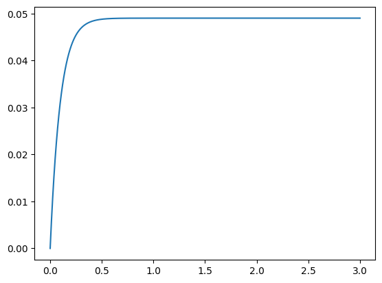
This is a very straightforward example with simple numbers to demonstrate using the functionality of the time solver. The system was not set up in a precise enough way to warrant any serious interpretation of the output (although it does visually settle into steady-state behavior), but we can see that it produces an object of type Solution, just like a steady-state solve. Although it is the same type of object, it has some new attributes, some of which are demonstrated below.
print(f"rho shape: {sol_norwa.rho.shape}")
print(sol_norwa.axis_labels)
print(len(sol_norwa.t))

susc_norwa=sol_norwa.coupling_coefficient_observable()
plt.plot(sol_norwa.t, susc_norwa.imag)
plt.show()
rho shape: (1000, 15)
['time', 'density_matrix']
1000
3.2 Initial conditions
Obviously, it does not make sense to discuss a time-domain solve without discussing the initial condition of the system. Since no explicit condition was defined in the above example, it begs the questions of 1. What intial condition was used? and 2. Is there any way to use a different one? Thankfully, there are simple answers to both questions. Let’s recreate the example 3.1.
#101 Mrad/s field, modulated
def my_field_norwa(t):
    return np.cos(101*t)*np.sin(10*t)

sensor_time_norwa = rq.Sensor(4)
sensor_time_norwa.add_coupling((0,1), detuning=0, rabi_frequency=1)
sensor_time_norwa.add_coupling((1,2), detuning=0, rabi_frequency=2)
sensor_time_norwa.add_coupling((2,3), transition_frequency=100, rabi_frequency=1, time_dependence=my_field_norwa)

sensor_time_norwa.add_transit_broadening(10)
sensor_time_norwa.add_decoherence((2,1), 1)
sensor_time_norwa.add_decoherence((3,2), 0.1)

#1000 samples over 3 microsecond
end_time = 3
num_pts = 1000

sol_norwa = rq.solve_time(sensor_time_norwa, end_time, num_pts)
Thankfully, the initial condition used is actually saved in the Solution object when solve_time is called under the init_cond attribute:
print(sol_norwa.init_cond)
[-0.         -0.00463991  0.          0.04905154  0.00478423 -0.
  0.         -0.          0.00066507  0.00012092  0.         -0.
 -0.         -0.         -0.        ]
This density matrix (remember that the basis of the density matrix is altered in rydiqule) is the steady-state solution of the system based on the Hamiltonian at time t=0, as we can see below. We will introduce the get_time_hamiltonian function, which is not crucial to know, but will demostrate where the result comes from.
print(sensor_time_norwa.get_time_hamiltonian(0))
print(rq.solve_steady_state(sensor_time_norwa).rho)
[[  0. +0.j   0.5+0.j   0. +0.j   0. +0.j]
 [  0.5+0.j   0. +0.j   1. +0.j   0. +0.j]
 [  0. +0.j   1. +0.j   0. +0.j   0. +0.j]
 [  0. +0.j   0. +0.j   0. +0.j 100. +0.j]]
[-0.         -0.00463991  0.          0.04905154  0.00478423 -0.
  0.         -0.          0.00066507  0.00012092  0.         -0.
 -0.         -0.         -0.        ]
So the steady-state solution (which uses the t=0 hamiltonian for a steady-state sole when there is a time-dependant coupling) is the same as the the initial condition.
Setting the intial condition manually is as simple as using the init_cond argument in rq.solve_time. In this case, we will demonstrate a simple case where all population is in the ground states. Remember that since rydiqule removes the ground state population when it solves, this corresponds to an array of zeros with length \(n^2-1 = 15\). If you would like a more involved intial condition, you can create the familiar square complex (hermitian) density matrix, and call rq.sensor_utils.convert_complex_to_dm() to get the corresponding real flattened density matrix.
all_ground = np.zeros(4**2-1)
sol_norwa_ground = rq.solve_time(sensor_time_norwa, end_time, num_pts, init_cond=all_ground)
susc_norwa_ground = sol_norwa_ground.coupling_coefficient_observable()

fig, ax = plt.subplots()
ax.plot(sol_norwa_ground.t, susc_norwa_ground.imag)
plt.show()
This plot helps shed some light on the reason rydiqule makes the default choice it does. The transient ramp up is much bigger, and it is hard to see any oscillations in this plot. Depending on what you are modelling, it often makes sense to leave the inital condition alone, but it is useful to know you can change it. Let’s chop off the first 340 points and see that the steady-state behavior is still similar:
fig, ax = plt.subplots()
ax.plot(sol_norwa_ground.t[340:], susc_norwa_ground.imag[340:]);
plt.show()

3.3 Time Dependance with the RWA
Now that we have shown time-dependence in the simplest case, with no rotating wave approximation, let us examine how we can still use the rotating wave approximation and still solve for time-domain behavior of the system. This is desirable in a number of cases, for example in a pulsed laser scheme.
Remember that if the RWA is valid for the system you are trying to model, it is generally a good idea to use it. rydiqule does note make any decisions regarding this for you, it is up to the physicist to decide in which situations it is a reasonable approximation of system behavior. In any time solver, modelling higher frequencies will be slower. Depending on how high your frequencies are, this can be many orders of magnitude. For this reason, modelling lasers fully in the time domain, for example is basically always a bad idea; you might be waiting an amount of time that is, practically speaking, forever.
Below we show a system that we define similarly to the previous example, the only exception being that the (2,3) coupling now is specified with a 1 Mrad/s detuning (the same detuning defined explicitly above), and show that the behavior is the same.
#101 Mrad/s field, modulated
def my_field_rwa(t):
    return np.sin(10*t)

sensor_time_rwa = rq.Sensor(4)
sensor_time_rwa.add_coupling((0,1), detuning=0, rabi_frequency=1)
sensor_time_rwa.add_coupling((1,2), detuning=0, rabi_frequency=2)
sensor_time_rwa.add_coupling((2,3), detuning=1, rabi_frequency=1, time_dependence=my_field_rwa)

sensor_time_rwa.add_transit_broadening(10)
sensor_time_rwa.add_decoherence((2,1), 1)
sensor_time_rwa.add_decoherence((3,2), 1)

print(sensor_time_rwa)

#1000 samples over 3 microsecond
end_time = 3
num_pts = 1000

sol_rwa = rq.solve_time(sensor_time_rwa, end_time, num_pts)
<class 'rydiqule.sensor.Sensor'> object with 4 states and 3 coherent couplings.
States: [0, 1, 2, 3]
Coherent Couplings:
    (0,1): {rabi_frequency: 1, detuning: 0, phase: 0, kvec: (0, 0, 0), coherent_cc: 1.0, label: (0,1)}
    (1,2): {rabi_frequency: 2, detuning: 0, phase: 0, kvec: (0, 0, 0), coherent_cc: 1.0, label: (1,2)}
    (2,3): {rabi_frequency: 1, detuning: 1, phase: 0, kvec: (0, 0, 0), time_dependence: <function my_field_rwa at 0x000002333D6FC9A0>, coherent_cc: 1.0, label: (2,3)}
Decoherent Couplings:
    (0,0): {gamma_transit: 10.0}
    (1,0): {gamma_transit: 10.0}
    (2,0): {gamma_transit: 10.0}
    (2,1): {gamma: 1.0}
    (3,0): {gamma_transit: 10.0}
    (3,2): {gamma: 1.0}
Energy Shifts:
    None
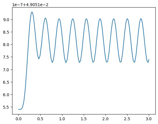
Just like before, we will print the imaginary part of a unitless “susceptibility” against time, and see that indeed we get similar transient and quick steady-state behavior.
fig, ax = plt.subplots()
susc=sol_rwa.coupling_coefficient_observable()
ax.plot(sol_rwa.t, susc.imag);
plt.show()
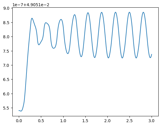
There is an important caveat with regards to how to think about RWA couplings in the time domain. Remember that the approximation treats the field in the rotating frame of the field. In rydiqule this applied field is implicitly assumed to be part of the coupling. This is how we keep specifications of couplings quick and easy. So in the above example, our 101 Mrad/s field is rotated into the 101 Mrad/s frame, with of 1 Mrad/s detuning from resonance (accounted for on the diagonal). As a result, the \(\cos(101t)\) field becomes 1 as far as rydiqule is concerned, and we are left only with the modulating \(\sin\) function and the manually specified detuning of 1 Mrad/s.
One should also note that there are some obvious numeric artifacts. Their origin and how to mitigate them is described in section 3.4.
Any python function works
Since rydiqule just calls the provided time function with no inference of its mathematical form, any python funtion will work; it need not be a sinusoid. This opens up options for things like stepwise functions. Lets reproduce the above RWA example, but rather than modulating the field by a sinusoid, we will use a pulsing function.
# off from 0 to 1, on from 1 to 2, repeat
def pulse_field(t):
    if 0 <= t%2 <= 1:
        return 0.0
    else:
        return 1.0

sensor_time_pulse = rq.Sensor(4)
sensor_time_pulse.add_coupling((0,1), detuning=0, rabi_frequency=1)
sensor_time_pulse.add_coupling((1,2), detuning=0, rabi_frequency=2)
sensor_time_pulse.add_coupling((2,3), detuning=1, rabi_frequency=1, time_dependence=pulse_field)

sensor_time_pulse.add_transit_broadening(10)
sensor_time_pulse.add_decoherence((2,1), 1)
sensor_time_pulse.add_decoherence((3,2), 1)

print(sensor_time_pulse)

#1000 samples over 1 microsecond
end_time = 10
num_pts = 1000
<class 'rydiqule.sensor.Sensor'> object with 4 states and 3 coherent couplings.
States: [0, 1, 2, 3]
Coherent Couplings:
    (0,1): {rabi_frequency: 1, detuning: 0, phase: 0, kvec: (0, 0, 0), coherent_cc: 1.0, label: (0,1)}
    (1,2): {rabi_frequency: 2, detuning: 0, phase: 0, kvec: (0, 0, 0), coherent_cc: 1.0, label: (1,2)}
    (2,3): {rabi_frequency: 1, detuning: 1, phase: 0, kvec: (0, 0, 0), time_dependence: <function pulse_field at 0x000002333D673600>, coherent_cc: 1.0, label: (2,3)}
Decoherent Couplings:
    (0,0): {gamma_transit: 10.0}
    (1,0): {gamma_transit: 10.0}
    (2,0): {gamma_transit: 10.0}
    (2,1): {gamma: 1.0}
    (3,0): {gamma_transit: 10.0}
    (3,2): {gamma: 1.0}
Energy Shifts:
    None
sol_pulse = rq.solve_time(sensor_time_pulse, end_time, num_pts)
susc_pulse = sol_pulse.coupling_coefficient_observable()

fig, ax = plt.subplots()
ax.plot(sol_pulse.t, susc_pulse.imag);
plt.show()
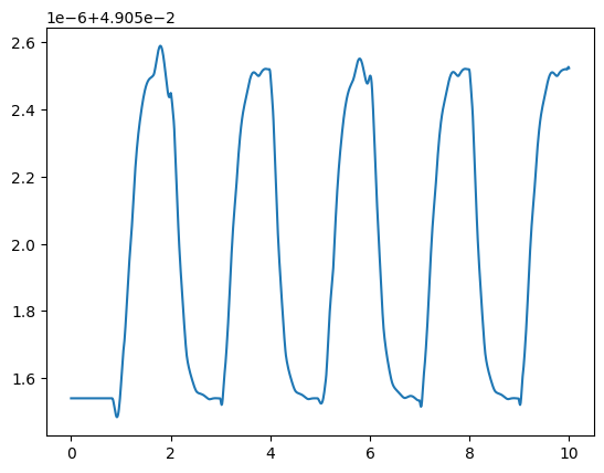
We did not leave enough time to enter a steady-state on any particular pulse (again, we are not trying to demonstrate meaningful physics in this notebook), but we can see that the solver ran fine, and the plusing behavior we would expect is present.
3.4 Multi-value Parameters in a time solve
Just like solve_steady_state, solve_time supports coupling parameter definitions that are list-like. It works more or less as you might expect based on the behavior of steady-state solving, but it is worth briefly discussing for the sake of demonstrating what the solution might look like.
We will start with a Sensor identical to the one in 3.3, but with the (2,3) transition’s rabi_frequency and detuning defined as lists. Note that because we are scanning 2 parameters over 51 values, there are actually \(51\times 51=2,601\) sets of equations being solved. rydiqule is pretty efficient, even in the time solver, for reasonable frequencies, but is not magical. This cell may take longer than previous ones (and probably spin up your computer fans a little), but it should be doable.
#101 Mrad/s field, modulated
def my_field_rwa(t):
    return np.sin(10*t)

dets = np.linspace(-5,5,51)
rabis = np.linspace(-1,1,51)

sensor_time_scan = rq.Sensor(4)
sensor_time_scan.add_coupling((0,1), detuning=0, rabi_frequency=1)
sensor_time_scan.add_coupling((1,2), detuning=0, rabi_frequency=2)
sensor_time_scan.add_coupling((2,3), detuning=dets, rabi_frequency=rabis, time_dependence=my_field_rwa)

sensor_time_scan.add_transit_broadening(10)
sensor_time_scan.add_decoherence((2,1), 1)
sensor_time_scan.add_decoherence((3,2), 1)

print(sensor_time_scan)

#1000 samples over 3 microsecond
end_time = 3
num_pts = 1000

sol_time_scan =  rq.solve_time(sensor_time_scan, end_time, num_pts, atol=1e-9)

susc_scan = sol_time_scan.coupling_coefficient_observable()
<class 'rydiqule.sensor.Sensor'> object with 4 states and 3 coherent couplings.
States: [0, 1, 2, 3]
Coherent Couplings:
    (0,1): {rabi_frequency: 1, detuning: 0, phase: 0, kvec: (0, 0, 0), coherent_cc: 1.0, label: (0,1)}
    (1,2): {rabi_frequency: 2, detuning: 0, phase: 0, kvec: (0, 0, 0), coherent_cc: 1.0, label: (1,2)}
    (2,3): {rabi_frequency: <parameter with 51 values>, detuning: <parameter with 51 values>, phase: 0, kvec: (0, 0, 0), time_dependence: <function my_field_rwa at 0x000002333B4BD9E0>, coherent_cc: 1.0, label: (2,3)}
Decoherent Couplings:
    (0,0): {gamma_transit: 10.0}
    (1,0): {gamma_transit: 10.0}
    (2,0): {gamma_transit: 10.0}
    (2,1): {gamma: 1.0}
    (3,0): {gamma_transit: 10.0}
    (3,2): {gamma: 1.0}
Energy Shifts:
    None
As a note, we tightened our absolute tolerance on the time solver. Why is somewhat beyond the scope of this notebook, but it is worth briefly explaining. Under the hood, rydiqule uses scipy’s solve_ivp function with a Runge-Kutta method of order 4(5). To make this work seamlessly with large stacks, rydiqule performs some reshape operations, and with such a large vector, the "RK45" hueristics will behave differently on an huge list of values as opposed to just the 15 in a single density matrix.
The details are not relevant here, but these sorts of numerical analyses are something rydiqule can only take so far, you ultimately need to judge whether a potential numerical error has occured. We made the above choice by analyzing what the plot looked like. As a general rule, if the plot is behaving unexpectedly, the atol can be set an order of magnitude or so smaller than any oscillations. You may have astutely noticed that the RWA and non RWA examples above did not match exaclty, and this was almost certainly the reason. However, we made the decision not to adjust since we caputred the relevant behavior just fine. Ultimately, rydiqule uses the scipy default of 1e-3, but you may need to adjust it to suit your problem, just like you would with any ivp solver.
Anyhow, just as we did before, let us investigate some key parts of the Solution sol_time_scan:
print(sol_time_scan.rho.shape)
print(sol_time_scan.axis_labels)
(51, 51, 1000, 15)
['(2,3)_detuning', '(2,3)_rabi_frequency', 'time', 'density_matrix']
So we can see that the shape is as expected. The ordering of the time axes here is general – in a rydiqule time soluion, axes will always be ordered as parameters, time, density matrix.
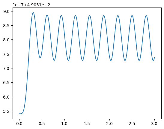
Just for fun, lets try and plot the solution, that corresponds to the single-value solve above, at detuning=1 and rabi_frequency=1. We use np.where() to get the correct indeces. Note that we can still apply functions like observales to the solution without changing the indexing
det_idx = np.where(dets==1)[0][0]
rabi_idx = np.where(rabis==1)[0][0] #the return typle of where is tuple(array), although there is only 1 index

time = sol_time_scan.t
print(susc_scan.shape)
susc_plot = susc_scan[30,50] #apply squeeze operatiob because indexing leaves
(51, 51, 1000)
fig, ax = plt.subplots()
ax.plot(time, susc_plot.imag)
plt.show()
3.5 Compiled timesolver backend
With version 2.2.0, rydiqule introduced a fully compiled timesolver backend: cyrk_solve.
This backend is written in cython and leverages CyRK’s cysolve_ivp.
It is generally faster than the default scipy backend by around an order of magntiude,
but requires that the time-dependence functions be compiled with cython by hand (including having a local C compiler).
No other aspect of Sensor creation or time-solving changes,
and the time-function compilation is readily achieved in a jupyter notebook,
as will be shown below.
Further details on cyrk_solve usage are in the API Docs.
A detailed exploration of the performance relative to the scipy backend
is located in an example notebook.
Note that the following three cells require that an appropriate C/C++ compiler and OpenMP library is installed on the system.
%load_ext Cython
%%cython
# cython: initializedcheck=False, cdivision=True, nonecheck=False, boundscheck=False, wraparound=False

from libc.math cimport sin
# have to use complex math functions from here to avoid MSVC C99 shenanigans
from rydiqule.stack_solvers.cyrk_solver.complex cimport double_complex
from rydiqule.stack_solvers.cyrk_solver cimport tfunc_wrapper

cdef double complex my_field_rwa_cy(double t) noexcept nogil:
    cdef double s = sin(10*t)
    return double_complex(s, 0.0) # must use double_complex(real, imag) to define complex numbers

wrapped_rwa_cy = tfunc_wrapper(my_field_rwa_cy)
sensor_time_rwa_cy = rq.Sensor(4)
sensor_time_rwa_cy.add_coupling((0,1), detuning=0, rabi_frequency=1)
sensor_time_rwa_cy.add_coupling((1,2), detuning=0, rabi_frequency=2)
sensor_time_rwa_cy.add_coupling((2,3), detuning=1, rabi_frequency=1, time_dependence=wrapped_rwa_cy)

sensor_time_rwa_cy.add_transit_broadening(10)
sensor_time_rwa_cy.add_decoherence((2,1), 1)
sensor_time_rwa_cy.add_decoherence((3,2), 1)

print(sensor_time_rwa_cy)

#1000 samples over 3 microsecond
end_time = 3
num_pts = 1000

sol_rwa_cy = rq.solve_time(sensor_time_rwa_cy, end_time, num_pts, solver='cyrk')
<class 'rydiqule.sensor.Sensor'> object with 4 states and 3 coherent couplings.
States: [0, 1, 2, 3]
Coherent Couplings:
    (0,1): {rabi_frequency: 1, detuning: 0, phase: 0, kvec: (0, 0, 0), coherent_cc: 1.0, label: (0,1)}
    (1,2): {rabi_frequency: 2, detuning: 0, phase: 0, kvec: (0, 0, 0), coherent_cc: 1.0, label: (1,2)}
    (2,3): {rabi_frequency: 1, detuning: 1, phase: 0, kvec: (0, 0, 0), time_dependence: <rydiqule.stack_solvers.cyrk_solver.utils.Tfunc_Wrapper object at 0x0000023353ECF1D0>, coherent_cc: 1.0, label: (2,3)}
Decoherent Couplings:
    (0,0): {gamma_transit: 10.0}
    (1,0): {gamma_transit: 10.0}
    (2,0): {gamma_transit: 10.0}
    (2,1): {gamma: 1.0}
    (3,0): {gamma_transit: 10.0}
    (3,2): {gamma: 1.0}
Energy Shifts:
    None
fig, ax = plt.subplots()
susc=sol_rwa_cy.coupling_coefficient_observable()
ax.plot(sol_rwa_cy.t, susc.imag);
plt.show()
4. Simulating Doppler broadening
One final key piece of functionality in rydiqule is the ability to simulate a doppler-broadened system. Internally, this is handled by breaking a doppler velocity profile into some number of slices, then applying the corresponding detunings for each class to the unshifted solution. This produces many sets of equations of motion, which are then solved, and then a weighted average performed to get the doppler-broadened solution.
To set up a system with doppler broadening, we use the the "kvec" keyword the couplings definition along with the vP attribute. A kvec is a 3-element spatial vector corresponding to the usual definition of a k-vector for an electromagnetic plane wave, defined in units of Mrad/m. Sensor.vP is an attribute that defines the most probable speed for an atom in a given sensor assuming a 3-D Maxwell-Boltzmann velocity distribution. Note that when multiplied vP and kvec correspond to the most probable doppler shift vector with respect to a given laser in Mrad/s.
Configuring doppler settings can get involved, and much of the functionality surrounding doppler handling is beyond the scope of an introductory notebook. This will be a quick discussion, but should at least be useful in handling most simple cases. If applying the steps outlined here produces unexpected results, you can find more details about how rydiqule does doppler in the physics and api doppler documentation.
Note that as of version 2.1.0, in addition to solve_steady_state below, rydiqule supports analytic doppler averaging. More details of this function can be found in physics and api documentation.
4.1 A simple doppler example.
Let us recreate the system in 2.4 above, which was the first thing we plotted. Recall that there was a large main peak, consisting of 3 sharp subpeaks. If we account for a small amount of doppler, broadening, we would expect those sharper features to be smeared out. In the example below we will apply doppler broadening to a pair of co-propagating lasers.
A doppler broadening of 1 MHz is wider than the narrow subpeaks but narrower than the main peak, so with that amount of broadening, the large peak should stay similar in width, but the small peaks will no longer be able to be resolved. Let us test this hypothesis as a quick smell-check that rydiqule is doing something reasonable with doppler broadening.
Recall that kvec is an attribute of a particular coupling, while vP is a property of sensor, and can be defined either in the constructor using Sensor(....,vP=<value>), or after construction with my_sensor.vP = <value>
basis_size = 4
sensor_doppler = rq.Sensor(basis_size, vP=2)

k_mag = np.pi #Mrad/m
k_direction = np.array([1,0,0])

detunings = 2*np.pi*np.linspace(-10,10,201) #201 values between -10 and 10 MHz
probe = {"states":(0,1), "detuning": detunings, "rabi_frequency": 3, 'kvec': k_direction*k_mag}
coupling = {"states":(1,2), "detuning": 0, "rabi_frequency": 5, 'kvec': k_direction*k_mag}
rf = {"states":(2,3), "detuning": 0, "rabi_frequency":7}

sensor_doppler.add_couplings(probe, coupling, rf)

gamma = np.zeros((basis_size, basis_size))
gamma[1:,0] = 0.1
sensor_doppler.set_gamma_matrix(gamma)

print(sensor_doppler)
<class 'rydiqule.sensor.Sensor'> object with 4 states and 3 coherent couplings.
States: [0, 1, 2, 3]
Coherent Couplings:
    (0,1): {rabi_frequency: 3, detuning: <parameter with 201 values>, phase: 0, kvec: <parameter with 3 values>, coherent_cc: 1.0, label: (0,1)}
    (1,2): {rabi_frequency: 5, detuning: 0, phase: 0, kvec: <parameter with 3 values>, coherent_cc: 1.0, label: (1,2)}
    (2,3): {rabi_frequency: 7, detuning: 0, phase: 0, kvec: (0, 0, 0), coherent_cc: 1.0, label: (2,3)}
Decoherent Couplings:
    (1,0): {gamma: 0.1}
    (2,0): {gamma: 0.1}
    (3,0): {gamma: 0.1}
Energy Shifts:
    None
Before checking out the solution, Let us briefly touch on what is happening under the hood with a doppler solve. rydiqule leverages its existing stack framework internally by adding more hamiltonians to the stack. It will create and solve a set of Hamiltonians and equations for each doppler class. Then at the end, it will apply weights based on the population in each class assuming a Boltzmann distribution of velocity classes, and sum the weighted classes together. Note that the solution’s final shape is the same as it would be without doppler. So the internals of dopper are, in basic cases, something you don’t actually need to see.
Note that since doppler is a parameter of the solve rather than an argument of Sensor itself,
solution_doppler = rq.solve_steady_state(sensor_doppler, doppler=True)
print(f"Solution shape: {solution_doppler.rho.shape}")
Solution shape: (201, 15)
absorption_doppler = solution_doppler.coupling_coefficient_observable().imag
plt.plot(detunings, absorption_doppler)
plt.show()
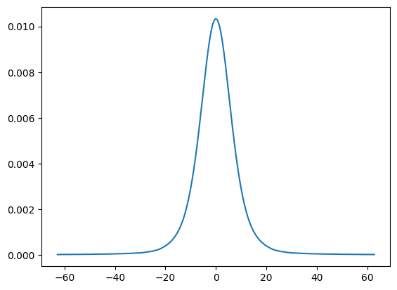
Perfect, it is as we expected: The three narrow peaks comprising the larger one have been blurred into a single peak.
It is also worth mentioning that the same argument works identically in the solve_time() function.
4.2 A word of caution
Once you realize rydiqule can do doppler broadening, it may be tempting to apply it to all your experiments. It is important to keep in mind that for each axis over which you account for doppler broadening, you are increasing the number of equations to solve by a factor of \(n_{classes}\), which by default is ~600. Remember, in its current iteration rydiqule explicitly solves every doppler class, it does not use any hueristics. Adding doppler broadening can quickly get out of control in both memory and computation time. A seemingly innocuous kvec=k_mag*(1,1,1) will apply doppler broadening in 3 dimensions and increase the number of equations rydiqule solves by a factor of 8,000,000. This is not to tell you not to use doppler, just to understand what you are asking rydiqule to do.
5. What Next?
Hopefully, you now have a good idea of the basics of how rydiqule can be used to solve atomic systems in a variety of ways. Depending what you want to do, you can start running your own simulations.
If you intend to simulate real-world lab experiments with actual Rydberg atoms, the rydiqule.Cell module has tools to do exaclty that. It inherits from Sensor, so all the basic priciples apply, but some funcitonality has been added to calulate things like dipole moments, decay rates, and state energies automatically using functionality from the ARC package. We have a Cell_Basics.ipynb notebook in the same folder as this one, and you now equipped to go through that tutorial. That notebook will assume that you understand the principles of this one, but it provides useful tools to start simulating your own Rubidium. After that, the rest of the examples in this notebook show examples using Cell to simulate real experiments that you could do in a lab.